Comparison of SNP detection using duplicate sequencing runs in SNiPgenie
Background
Whole genome sequence data is now commonly used for bacterial epidemiology. For clonal species, the typical method is the ‘map to reference and SNP site analysis method’. The reads are aligned to a reference genome, variants called and filtered. From this shares SNP sites are identified. The base at each site for all samples are then placed in a fasta file which is basically a sequence alignment. This can be used to build a phylogeny. Ideally we can detect a difference of even a single SNP between two related species. To test this we used two independent sequencing runs for 16 M.bovis isolates. Libraries were prepared separately from the same cultures. Illumina sequencing was performed on two different platforms, a NextSeq 500 with 150 paired end reads and a MiSeq with ~250-300 paired end reads.
The data was then analysed in SNiPgenie by running all samples together and then retrieving the SNP distance matrix and maximum likelihood tree. From this we could compare the SNP distance between each corresponding pair, which should be zero. The code is available here.
Results
SNiPgenie has filters normally used with our M.bovis samples. One is a proximity filter that excludes SNPs within 10 bp of each other. The other is to mask all sites within genes with repeat regions, a common source of false positive calls. The comparison was run with and without the filters. Normal quality filters were retained since these are always used anyway. The plot below shows the SNP distances for each pair of runs for a sample. It is seen that without filters we often get more differences. In some cases up to 5 SNPs. Note that the bottom three samples are probably identical to each other. Even with filters we occasionally see 1 or 2 SNPs differences which can therefore be taken as the lower limit of our ability to detect genuine differences.
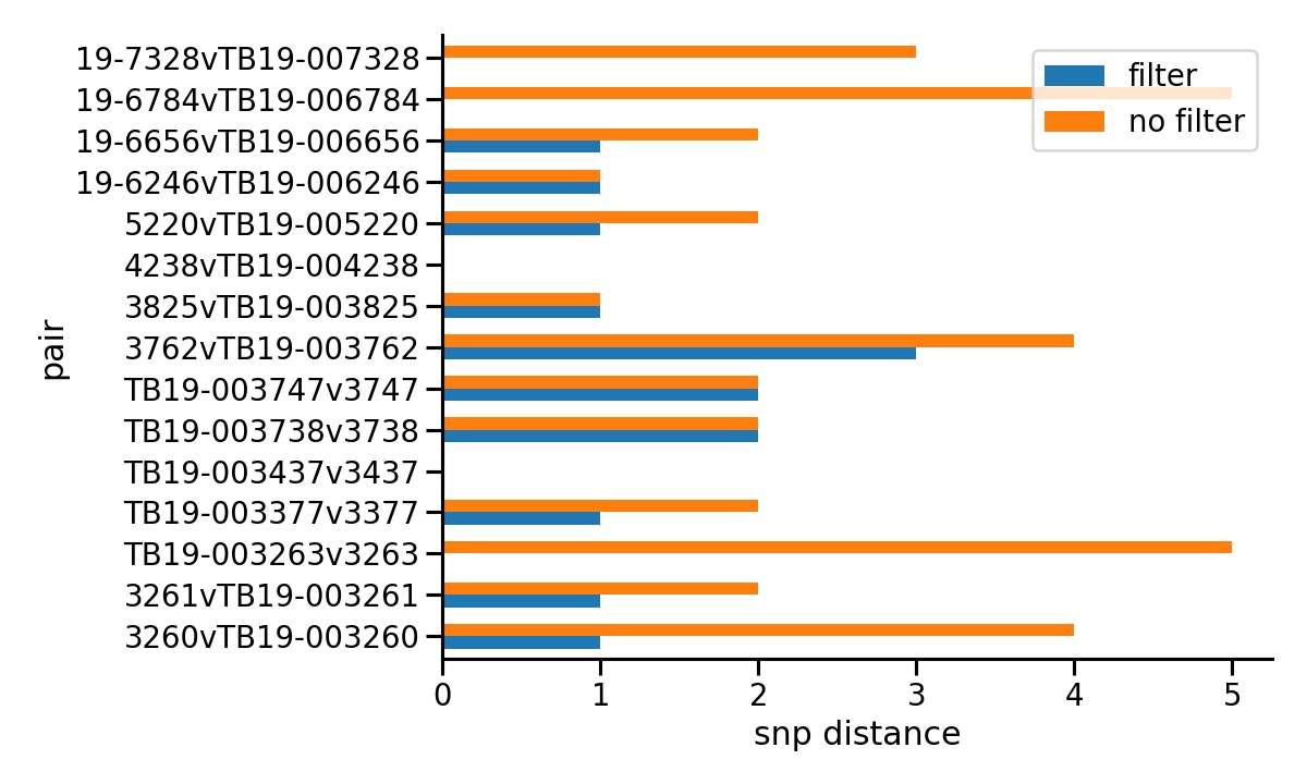
SNP distance between pairs of duplicates.
Trees
We can also see the effect of the filters on the resulting phylogeny generated from the SNP alignment.
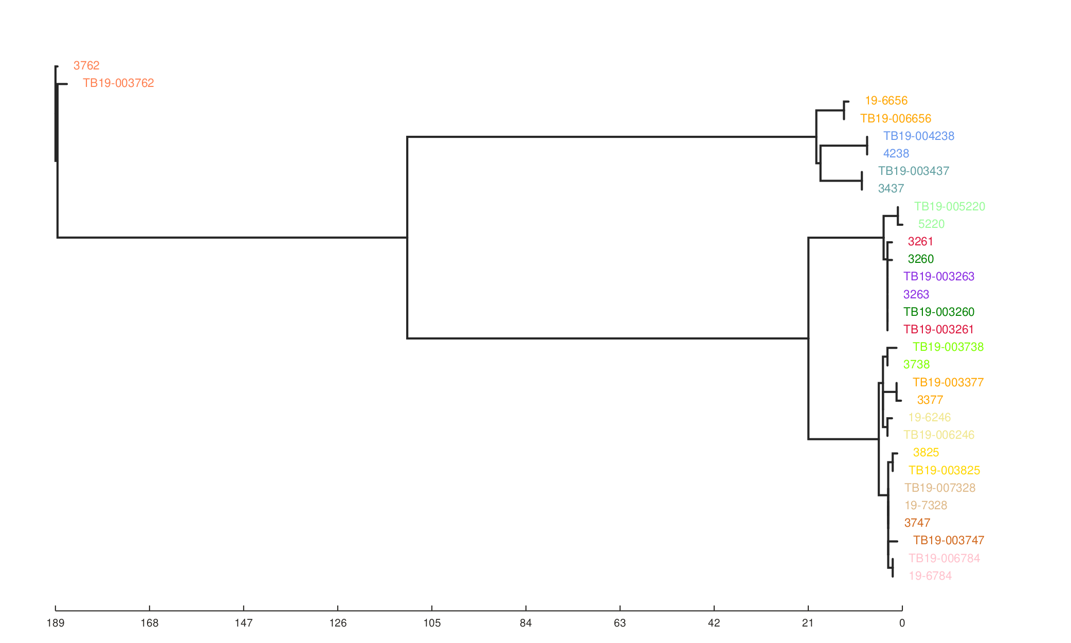
ML tree from SNP sites with all filters used.
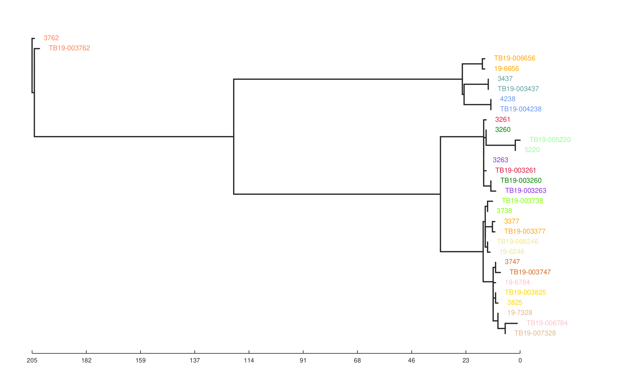
Tree without filters.
Where are these SNPs?
Some of the SNPs from the unfiltered run are due to PE/PPE genes that are normally masked. If we look at the locations of the filtered SNPs a number of sites appear repeatedly across multiple samples in different parts of the phylogeny. This indicates they are false positives. On closer inspection we see that the sites in the protein Mb2038c are due to a problematic homologous region in the protein that also maps to Mb1794c. The majority of sites are in this region in fact. It is possible that some of these regions should be masked along with the repeat regions.
Different SNPs called due to multimapping reads in homologous regions.
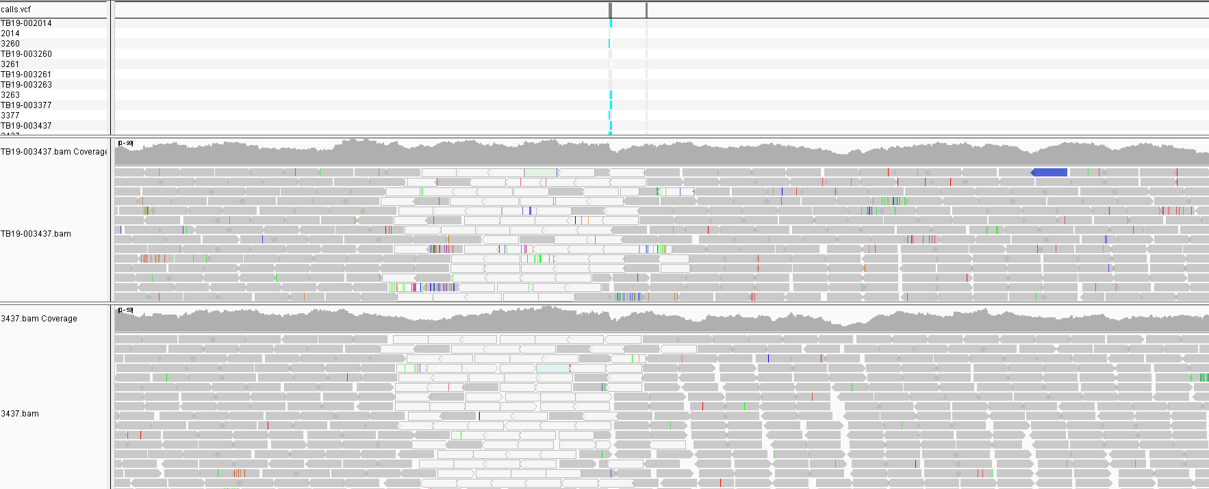
Another site that appears in one sample is in the pckA gene and appears possibly real. There is no call in the lower sample perhaps due to it’s low coverage. So differential coverage could certainly cause these differences to appear and a low coverage sample might be prone to missing a site that is actually present.
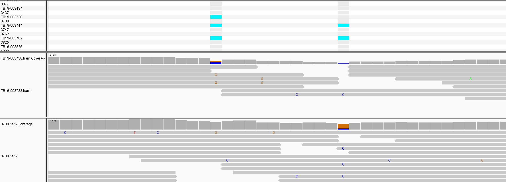
Different SNPs called on two identical samples due to different coverage.