SNP clustering and type naming of pathogens from WGS
Background
Whole genome sequencing (WGS) has emerged as a powerful tool in the field of public health, specifically in the context of pathogen strain typing. In order to categorize strains they are traditionally ‘typed’ using molecular methods like spoligotyping, MIRU-VNTR, RFLP or MLST. With WGS this can be accomplished at a superior resolution. WGS provides a detailed blueprint of virtually the entire genome. This allows every SNP difference between samples to be counted, within the error of instrument measurement. This information is used to help track the transmission and spread of infectious diseases or identify the source of outbreaks. Often WGS is used to assemble genomes and count alleles of reliable predefined genes, a type of whole genome MLST (wgMLST). This offers standardization and effectively avoids problems associated with genes moving in and out of the genome in many species, where SNPs calling would be made complex. For ‘clonal’ bacteria like TB, which generally change quite slowly by single nucleotide mutations, it is possible to count all the SNPs from variant calling and count the differences.
In either case, for general surveillance it is necessary to create a naming scheme that reflects the grouping of strains. A straightforward solution is to create a hiercharchical system where strains are assigned common ‘lineages’ based on their relatedness at a given threshold level. Different levels can be used to compose the strain name down to a high resolution level, thus creating a consistent nomenclature. This should also be dynamic to accomodate new strains as they are added to the known population. This concept is not new. Such a system has already been described and implemented in the SnapperDB tool 1. Another is the Pango lineage designation system used for Sars-Cov-2.
A method is given here, implemented in Python, that makes a naming scheme by clustering at given SNP levels and allows new samples to be added in batches. It uses agglomerative clustering to cluster samples according to their SNP distance.
Method
The method here is as follows:
- get core alignment for baseline population i.e. from variant calling
- generate SNP distance matrix
- cluster samples using distance matrix using agglomerative (single linkage) clustering such that such that all members of a cluster are within n SNPs of each other
- retain cluster membership and numbering for next run
For subsequent runs:
- get core alignment for new samples and combine with the previous (master) one
- compute new distance matrix
- cluster again applying old cluster labels
- store new clusters
This means we must always retain a ‘master’ copy of the core SNPs and cluster labels. Preferably also keep the SNP matrix to avoid recomputing the entire matrix every time a new sample is added. The method is summarised below.

Code
Here is code for testing this method. It first makes a simulated set of sequences that acts as the ‘core SNP aligmnent’ we would use in real data. This is derived from a simple Agent based model that gives us a phylogeny and distance matrix. You can also provide these as output from a real variant calling program and read them in as pandas dataframes. The newick tree is used to illustrate the results below and is not a requirement.
import pandas as pd
from btbabm import models,utils
from snipgenie import clustering,tools,plotting
import toytree

#make some simulated data
model = models.FarmPathogenModel(F=20,C=400,S=8,seq_length=500)
model.run(500)
#get metdata from model, will also write a newick tree
gdf, snpdist, meta = model.get_metadata(treefile='cluster_test/tree.newick')
X=meta.set_index('id')[['species','strain']]
To test the functionality we make a subset of the simulated data and run the clustering on the this. We then add more samples and run the clustering again, using the previous cluster information.
def get_subset(snpdist,X,n=10,seed=10):
    #subset dist matrix
    sub = list(snpdist.sample(n, random_state=seed).index)
    S = snpdist.loc[sub,sub]
    X=X.loc[sub]
    return S,X

#just get a subset of the original samples
#S1 is the distance matrix and X1 is a dataframe of samples with some meta data
S2,X2 = get_subset(snpdist,X,n=20)
S1,X1 = get_subset(S2,X2,n=15)
To get strain names we can cluster at all levels using the clustering.get_cluster_levels method. Then the strain name is composed of each cluster label at each level. The levels used are arbitrary. members1 is a dataframe with cluster labels at all threshold levels. This is used as input for subsequent runs.
#first run
cl,members1 = clustering.get_cluster_levels(S1, linkage='single')

#second run, using previous cluster info
cl,members2 = clustering.get_cluster_levels(S2,members1)
ST2 = clustering.generate_strain_names(cl)
ST2 = X2[cols].merge(ST2,left_index=True,right_index=True)
Example
After running the above the final ST2 table (a dataframe) looks like this. You can see how the strain names are made up of each cluster label. The actual strain names are up to the end user and could be changed by customising the clustering.generate_strain_names method. Cluster labels are assigned starting from 1 in the order the clustering alogrithm finds the data so they are arbitrary. In this case the higher threshold cluster levels are all the same because of the narrow set of samples.

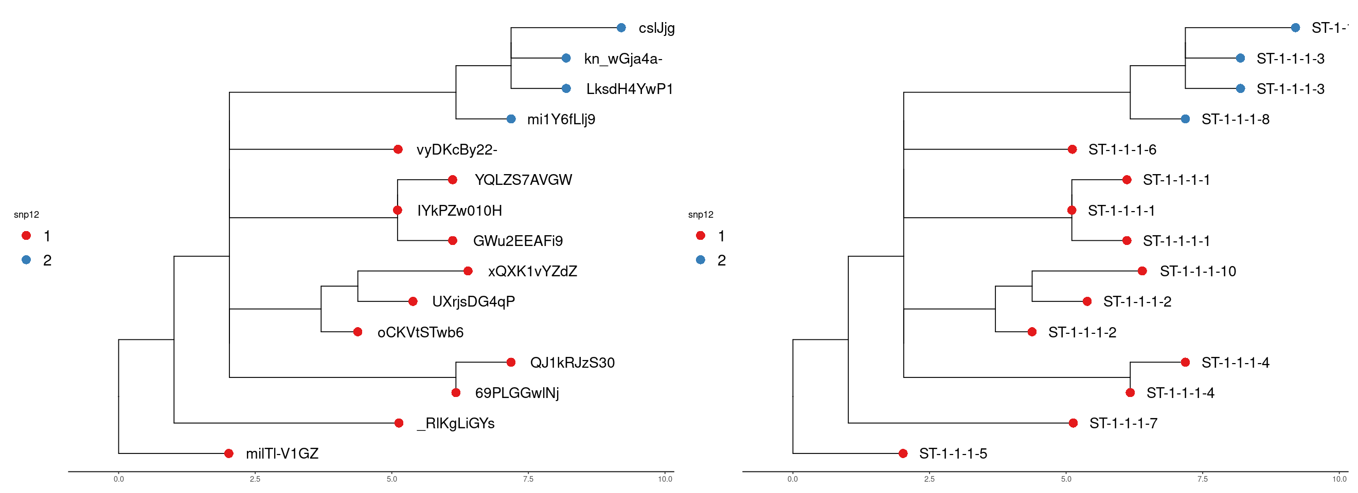
We can visualise the result using trees derived from the alignments. This lets us see the relationship of the clusters more easily. The tree is a neighbour-joining tree derived from the SNP distance matrix. The same tree is on the right with the strain names. The clusters are at the snp12 threshold.
Run 1
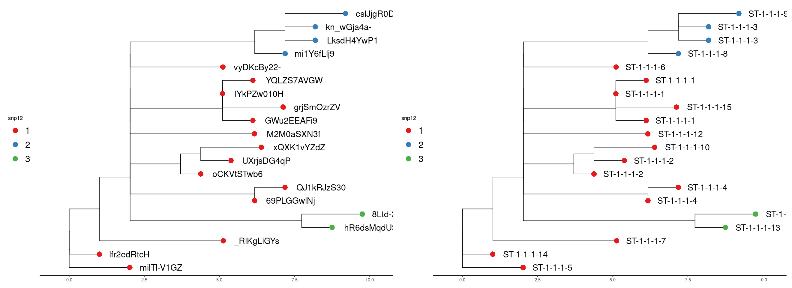
Run 2
In run 2 we can see the new samples have been added and the addition of a new cluster also.
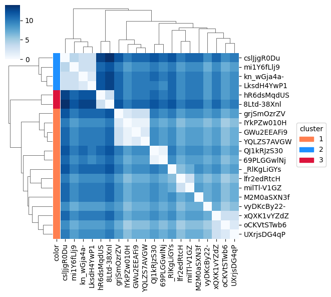
Clustermap of the same data:
Limitations
This method has some limitations in reality. When we run subsequent samples in a variant calling pipeline, some SNPs can drop out due to a low quality sample. This will create some inaccuracy. It just means we need quality control of input samples, particularly with regard to coverage. 98% coverage is a reasonable threshold for TB for example. The cluster allocation is also order dependent to some extent. It means adding new samples can occasionally alter cluster allocation and strain names will change accordingly.
The clustering code is available the SNiPgenie repository here.
Links
References
- SnapperDB: a database solution for routine sequencing analysis of bacterial isolates, Dallman et al. 2018 Bioinformatics https://doi.org/10.1093/bioinformatics/bty212
- “Automated Agnostic Designation of Pathogen Lineages”, McBroome et al. 2023. BioRxiv doi: https://doi.org/10.1101/2023.02.03.527052