Two quick ways of building a bacterial species phylogeny

March 22 2024

Background

Performing phylogenetic analysis with whole or core genome sequences maximizes the information used to estimate phylogenies and the resolution of closely related species. Usually sequences are aligned with a reference species or strain. However genome alignment is a process that does not scale well computationally. Even for small numbers of genomes it can be time consuming. Here are two relatively painless ways make a bacterial species phylogeny that you can do yourself. This might be useful if you are concerned with strains of a particular species you have sequenced and want to know how they relate to the nearest species in the genus.

In this example we will look at how the species in the Mycoplasmopsis genus are related. Mycoplasmopsis is a large genus among mollicutes and is of significant veterinary importance. You can see the taxonomy of the known species on NCBI but not a phylogeny. Note: There is a bit of confusion here as the mycoplasmopsis genus is a newer designation for some species formerly called Mycoplasma. The names are often used synonymously, i.e. Mycoplasma Bovis.

kSNP

kSNP4 is a program that identifies SNPs without doing alignments and a reference genome. This permits the inclusion of hundreds of microbial genomes that can be processed in a realistic time scale. Such an alignment free technique comes about through the insight that SNPs can be detected in small odd length chunks of sequence, kmers. So you split up the genomes into odd sized kmers and compare them. If the kmers are otherwise identical and are long enough not to be random, they can be compared between many samples to detect SNPs.

kSNP is mainly used for the analysis of viral and prokaryotic genomes. The input data are genome sequences in FASTA format. It can also annotate the SNPs if you include at least one annotation file. See more here.

Get genomes

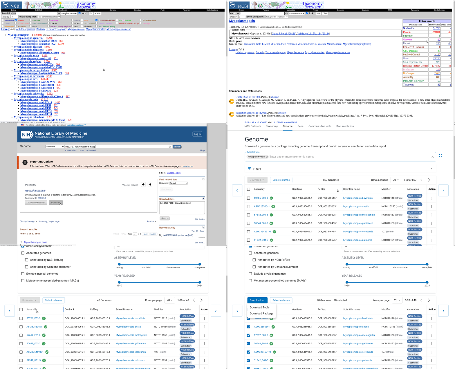
First we have to get the representative genomes of the genus (or a set of specific species). You can do this from the NCBI taxonomy browser here. This is the page for Mycoplasmopsis. Click on the genus name and it will show links to the genome page. You can follow the short screen capture below to see how to get the genome files. I filtered to only use reference genomes and retrieved 40. They don’t need to be completed/closed genomes for kSNP to work. Unzip the files.

Important: kSNP won’t accept names with a ‘.’ in them. Ours have so we have to rename the files first which is a bit annoying. We also need a flat file structure whereas the genomes assemblies are all placed in individual folders. I renamed them by just keeping the assembly ID.

To use kSNP there are basically three commands you need to run. They are shown below.

Make ksnp file (this is the input to the main program):

/local/kSNP4.1/MakeKSNP4infile -indir mycoplasmopsis_genomes/ -outfile ksnp_mycoplasmopsis.txt`

Use kchooser to determine the optimal kmer length. You will see it in the output. I got 19.

/local/kSNP4.1/Kchooser4 -in ksnp_mycoplasmopsis.txt

Finally, run kSNP4:

/local/kSNP4.1/kSNP4 -core -k 19 -outdir ksnp_mycoplasmopsis -in ksnp_mycoplasmopsis.txt

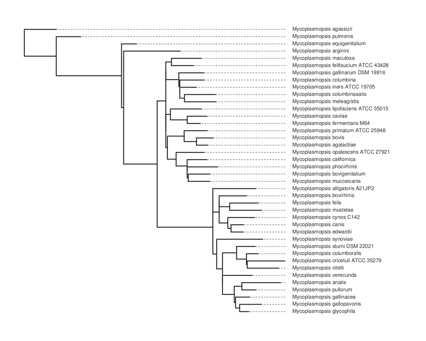
This will take maybe 10-15 minutes to run for about 80 genomes. It will produce a lot of files in the output folder. The one we want is the ML tree, tree.parsimony.tre. You can plot the tree using whatever program you wish. Here we use toytree, a Python package:

Here’s the code for the plot above. To get the species names we have to substitute them for the assembly name that’s used in the tree. We do this by loading the data_summary.tsv table that came with the download. This has a mapping between both and we use the ‘Organism Scientific Name’ field instead.

tre = toytree.tree('ksnp_mycoplasmopsis/tree.parsimony.tre')
tre = tre.root('GCF_002272945')
df = pd.read_csv('data_summary.tsv',sep='\t',index_col=5)
idx = tre.get_tip_labels()
df = df.reindex(index=idx)
df = df.loc[idx]
tiplabels = list(df['Organism Scientific Name'])
tre.draw(tip_labels_align=True, layout='r', tip_labels=tiplabels, width=900)
#save it
import toyplot.pdf
toyplot.pdf.render(canvas, "tree-plot.pdf")

Aside: FastANI

You can also use fastaANI to get a similarity (identity) measure between genomes. This also doesn’t use alignments. However it will not return values for genomes with <80% similarity, so should generally be used for fairly similar species or within species comparisons. To use this for many to many comparisons you make a list of all the fasta files in identical two seperate files, then supply these at the command line as follows:

fastANI --ql query1.txt --rl query2.txt -o fastani.out -t 8 --matrix

--matrix will output identity values arranged in a phylip-formatted lower triangular matrix format. This can easily be plotted.

Conserved proteins with OrthoDB

This option doesn’t really require whole genomes. You only really need one or several conserved genes from your species. It uses the OrthoDB site to find orthologs of a conserved protein and then aligns them the usual way. Single gene amino acid alignments are easy to do. Note that this method will likely not be sensitive enough to distinguish strains. Though you could use multiple genes joined together. The genes used might depend on what you want but normally they should be well conserved. 16S or other ribosomal subunits are often used to delineate species. You could also do this using Uniprot but this way is faster.

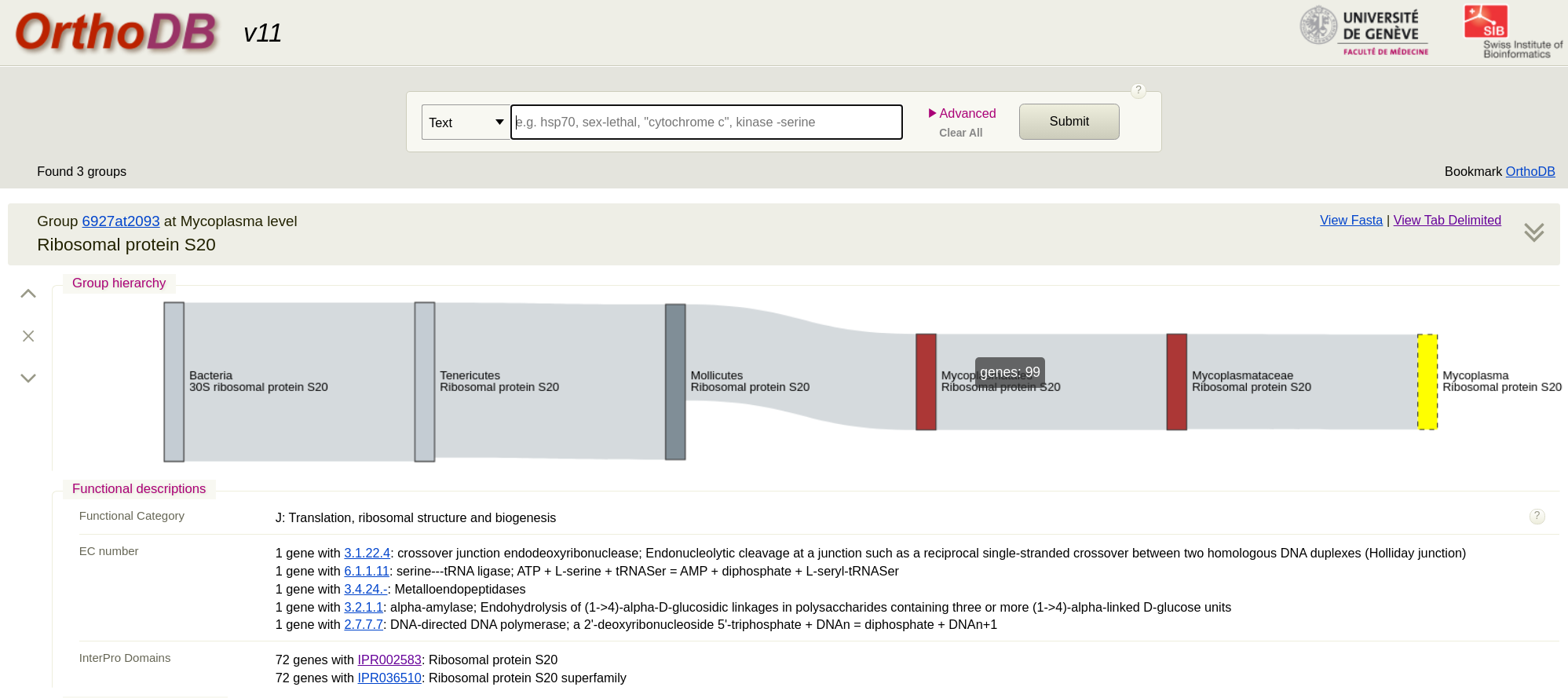
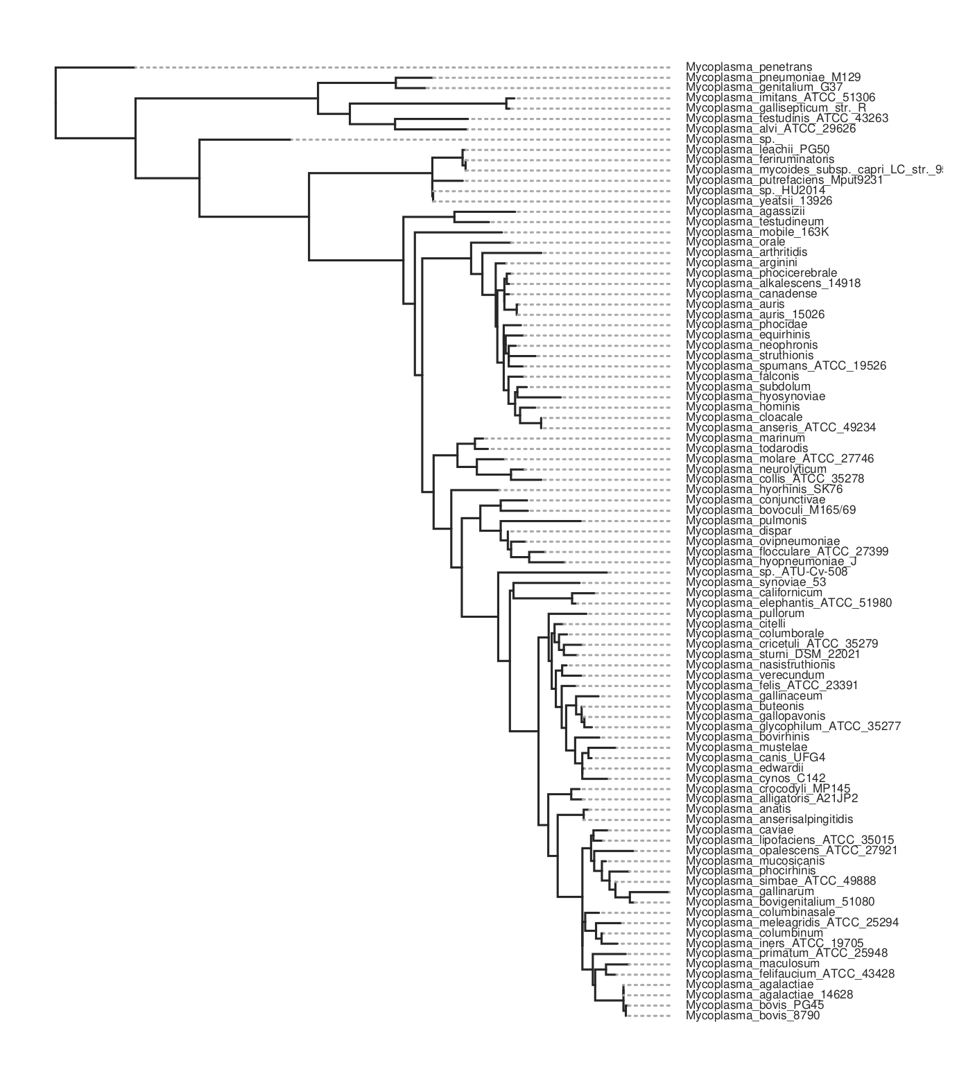
First we go to the OrthoDB site and search for a protein such as ‘Ribosomal protein’. This will give you lots of results and you can see they are grouped by genus level. Pick the Mycoplasma level for the protein you want. (The taxonomy here is not up to date for this genus). I picked Ribosomal protein S20. You will see that there are 98 sequences in the result. Just click on ‘view fasta’ to download the sequences. Remember these are amino acid sequences. To add your own strain to this from WGS data you would assemble the genome, run annotation tool like Prokka and extract the protein sequence. Then add it to the fasta you downloaded.

We then just have to align these sequences and make a tree. You will notice the fasta file has long headers with lots of fields. Here is some Python code that will simplify the headers and extract just the species name:

from Bio import SeqIO
from Bio.SeqRecord import SeqRecord
import json

#convert orthodb format to get species name only
new = []
found = []
for r in recs:
    x = r.description    
    #get the dict from the header
    data = json.loads(x.split(r.id)[1])     
    org = data['organism_name'].replace(' ','_')    
    if org in found:
        continue
    found.append(org)
    new.append(SeqRecord(id=org,seq=r.seq))
SeqIO.write(new,'mycoplasmopsis_S20_org.faa','fasta')

We can now align the sequences, this example uses mafft:

mafft mycoplasmopsis_S20_org.faa > out.aln

Make alignment with fasttree:

fasttree out.aln > out.tree

Here is the resulting tree. You can see there are more species than in the kSNP example above.

There is a Jupyter notebook here with this code.

References

Chan, J.ZM., Halachev, M.R., Loman, N.J. et al. Defining bacterial species in the genomic era: insights from the genus Acinetobacter. BMC Microbiol 12, 302 (2012). https://doi.org/10.1186/1471-2180-12-302
James T Stale. The bacterial species dilemma and the genomic–phylogenetic species concept. Phil. Trans. R. Soc. B 2006 DOI: 10.1098/rstb.2006.1914

category:
bioinformatics 52