Detecting polymorphisms in the RD900 region of MTBC species
Background
We have just published a paper detailing variation across the Mycobacterium tuberculosis Complex (MTBC) in the RD900 region. This region was first described as a lineage specific locus in M. africanum GM041182 strain (Bentley et al. 2012) and was thought to be deleted in M. bovis and “modern” M. tuberculosis lineages. RD900 region was not present in the original M. bovis AF2122/97 reference genome annotation, but was found to be actually present upon resequencing. These species show more than 99% genetic identity but exhibit distinct host preference and virulence. Differences in key locii are likely to be important in determining this.
The RD900 region comprises two homologous genes, pknH1 and pknH2, encoding a serine/threonine protein kinase PknH flanking the tbd2 gene. Our analysis revealed that RD900 has been independently lost in different MTBC lineages and different strains, resulting in the generation of a single pknH gene. Importantly, all the analysed M. bovis and M. caprae strains carry a conserved deletion within a proline rich-region of pknH, independent of the presence or absence of RD900. We hypothesized that deletion of pknH proline rich-region in M. bovis may affect PknH function, having a potential role in its virulence and evolutionary adaptation.
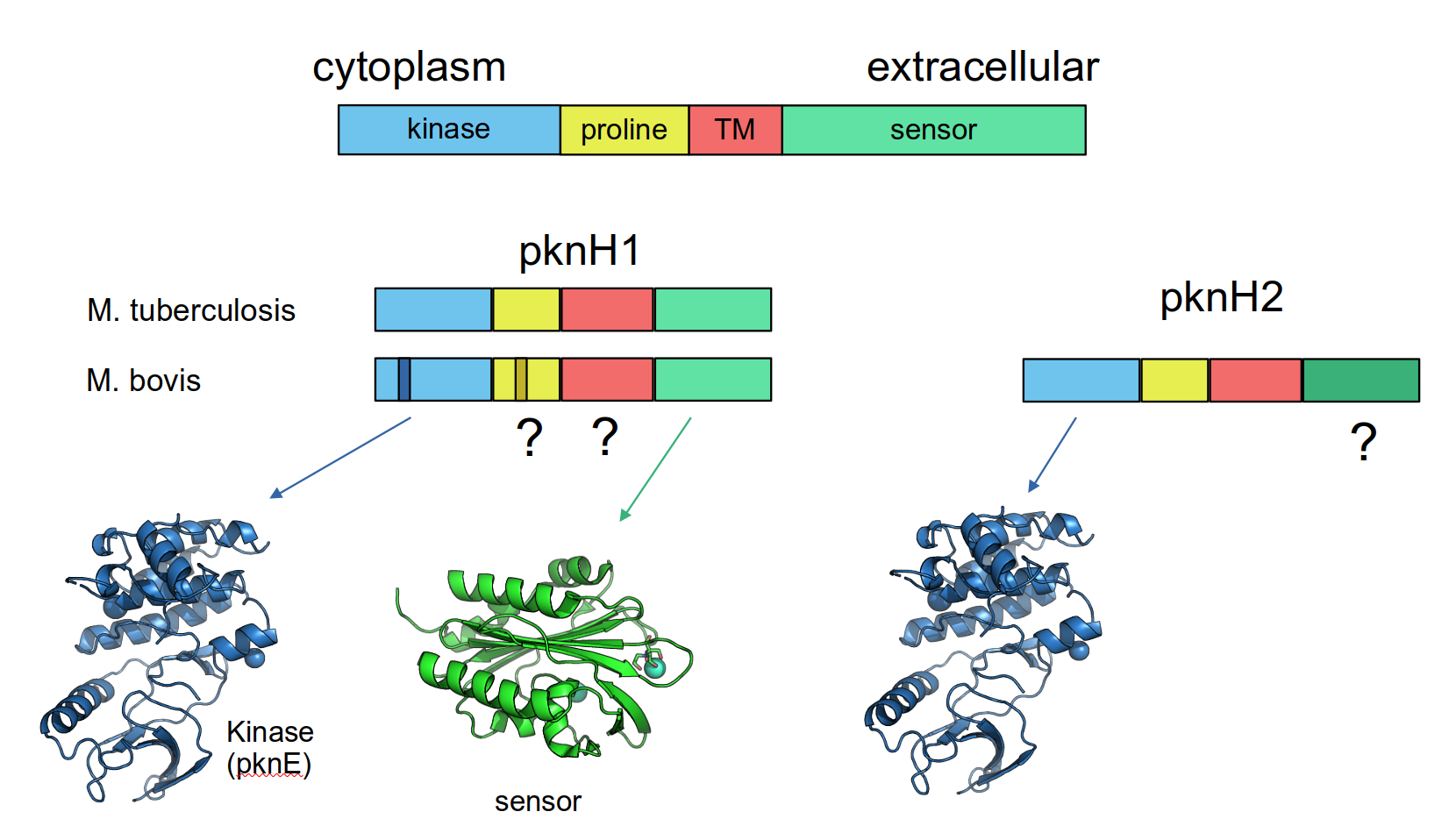
Structure of the pknH1 and pknH2 genes.
In this study we examined over 60 different MTBC strains representing lineages across the MTBC to see variations in the region. To accurately detect locus structure we used the raw read data instead of relying on assembled genomes which may have errors due to homology in the kinase domains of the pknH proteins, if both are present. Raw fastq files for all strains were downloaded and aligned to the most complete version of the RD900 locus encoded in the Mycobacterium africanum (MAF) genome. This allowed missing features to be seen as gaps, as shown below.
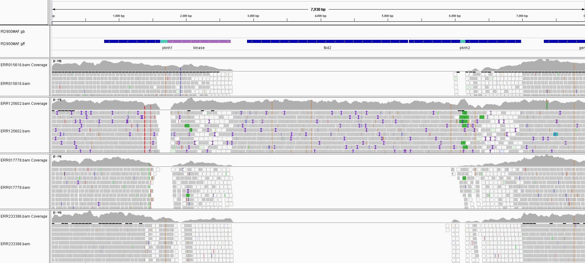
Alignments of some samples to the RD900 MAF region show the gaps where features are missing. The white reads are those multi-mapping to the homologous kinase domains of pknH1. This is what causes issues in assembly at this locus.
Automatic detection
Below is the code that tries to automatically determine the variation for many samples rather than visually inspect each alignment as we did in our study. This code is very specific to the problem in question but it (or part of it) may be of use for other similar applications. It can also be found in a Jupyter notebook in this repository.
Code
import os, io, glob, subprocess
from importlib import reload
from Bio import SeqIO
from Bio.SeqRecord import SeqRecord
from Bio.SeqFeature import SeqFeature, FeatureLocation
from BCBio import GFF
import numpy as np
import pandas as pd
import pylab as plt
import seaborn as sns

#read the table of sample info
read_data = pd.read_csv('../genomes_data.csv')
#load the locus features into a seqrecord
rec = list(GFF.parse('RD900MAF.gff'))[0]
Align the samples to the locus
This code uses the snpgenie package to conveniently perform alignment of the fastq files in one go. It’s normally used for variant calling as well but we can just use the alignment part. This tool can be called at the command line ot via Python as below.
from snpgenie import tools, aligners, app, trees, plotting

args = {'threads':20, 'outdir': 'snpgenie_results', 'labelsep':'-',
        'input':['/storage/raw_data/'],
        'reference': 'RD900MAF.fa',
        'overwrite':False
        }
W = app.WorkFlow(**args)
st = W.setup()
W.run()

samples = pd.read_csv('snpgenie_results/summary.csv')
samples = samples.merge(read_data,left_on='sample',right_on='ACCESSION')
samples = samples.sort_values('LINEAGE')
Detecting coverage across the locus
This method uses samtools to count coverage at each position in the alignment and saves it as a pandas DataFrame. We can then run for all samples.
def get_coverage(bam_file, chr, start, end):
    cmd = 'samtools mpileup {b} --min-MQ 10 -f RD900MAF.fa -r {c}:{s}-{e}'.format(c=chr,s=start,e=end,b=bam_file)
    temp = subprocess.check_output(cmd, shell=True)
    df=pd.read_csv(io.BytesIO(temp), sep='\t', names=['chr','pos','base','coverage','q','c'])
    return df
Plot the coverage
Here we use the method above to find coverage in each sample and plot them together.
from dna_features_viewer import GraphicFeature, GraphicRecord
from dna_features_viewer import BiopythonTranslator

graphic_record = BiopythonTranslator().translate_record(rec)
from matplotlib.gridspec import GridSpec
fig = plt.figure(figsize=(25,40))
gs = GridSpec(70, 1, figure=fig)
ax1=fig.add_subplot(gs[:3,0])
graphic_record.plot(ax=ax1)
i=3
for n,r in list(samples.iterrows()):
    ax=fig.add_subplot(gs[i,0])
    df = get_coverage(r.bam_file,'RD900MAF',1,len(rec.seq))
    df.plot(x='pos',y='coverage',ax=ax,kind='area',color='gray',legend=False)
    label=r.LINEAGE
    ax.text(-.12,.5,label,color='blue',transform=ax.transAxes,fontsize=12)
    ax.set_xticklabels([]); ax.set_yticklabels([])
    i+=1
plt.subplots_adjust(left=.3,right=.9,wspace=0, hspace=0)
fig.savefig('rd900_coverage.jpg',dpi=100)
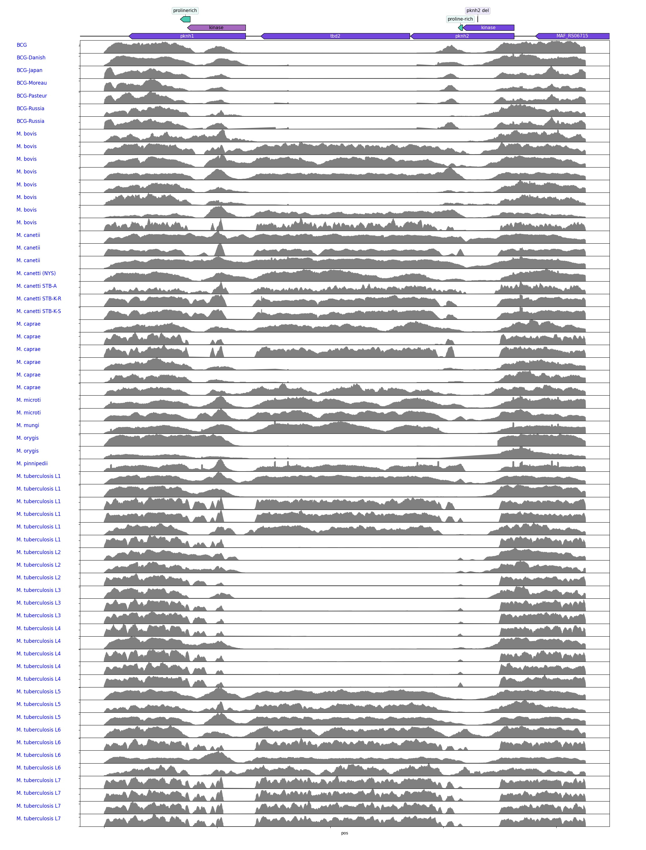
Coverage across the RD900 MAF region of all samples.
Automatically find presence/absence of features
As a bonus we can also try to automate the process of detecting the presence or absence of given features within the locus using the coverage data plotted above. We use the coords of each feature to find the average coverage which should be very low for those regions not covered by reads. This is the kind of thing that sounds good but doesn’t always work in practice. The clustermap below can be compared to the coverage map above for comparison.
def detect_coverage(file, ref, coords):
    """Find presence/absence within regions"""

    df = get_coverage(file,'RD900MAF',1,len(rec.seq)).set_index('pos')
    res=[]
    for c in coords:
        start,end=c[1],c[2]
        x = df.loc[start:end]
        x = (c[0],x.coverage.sum()/(end-start))
        res.append(x)
    return pd.DataFrame(res,columns=['region','coverage'])

#get the coordinates as tuples from the record features
coords = [(f.id,int(f.location.start),int(f.location.end)) for f in rec.features]
#or just provide them like this
coords = [('pknH1', 782, 2663),
 ('pknH1_proline', 1611, 1772),
 ('tbd2', 2906, 5303),
 ('pknH2', 5313, 6981),
 ('pknH2_proline', 6080, 6153),
 ('pknH1_kinase', 1725, 2663)]

#loop over all samples
M=[]
for i,r in list(samples.iterrows()):
    res = detect_coverage(r.bam_file,'RD900MAF.fa',coords)
    res['lineage'] = r.LINEAGE
    res['sample'] = r.ACCESSION
    M.append(res)
M=pd.concat(M)
#pivot the result
P = pd.pivot_table(M,index=['sample','lineage'],columns=['region'],values='coverage')
#set everything above/below a threshold to 1 or 0
P[P<1]=0
P[P>1]=1
This produces a table as shown below, which is essentially a presence/absence matrix for whatever feature coordinates we provide.
region                         pknH1  pknH1_kinase  pknH1_proline  pknH2  pknH2_proline  tbd2
sample     lineage
ERR015598  M. canetti STB-A      1.0           1.0            1.0    1.0            1.0   1.0
ERR015616  M. tuberculosis L2    1.0           1.0            1.0    1.0            0.0   0.0
ERR017778  BCG-Russia            1.0           1.0            0.0    1.0            1.0   0.0
ERR017801  M. tuberculosis L5    1.0           1.0            1.0    1.0            1.0   1.0
ERR027294  M. microti            1.0           1.0            1.0    1.0            0.0   1.0
ERR1109376 M. canetti STB-K-S    1.0           1.0            1.0    1.0            1.0   1.0
ERR1109377 M. canetti STB-K-R    1.0           1.0            1.0    1.0            1.0   1.0
ERR1200603 M. tuberculosis L7    1.0           1.0            1.0    1.0            1.0   1.0
ERR1200614 M. tuberculosis L4    1.0           1.0            1.0    0.0            0.0   0.0
ERR1200617 M. tuberculosis L7    1.0           1.0            1.0    1.0            1.0   1.0
Plot the result
cm=sns.clustermap(P,col_cluster=False,cmap='gray_r',figsize=(14,14),
                  xticklabels=True,yticklabels=True)
cm.cax.set_visible(False)
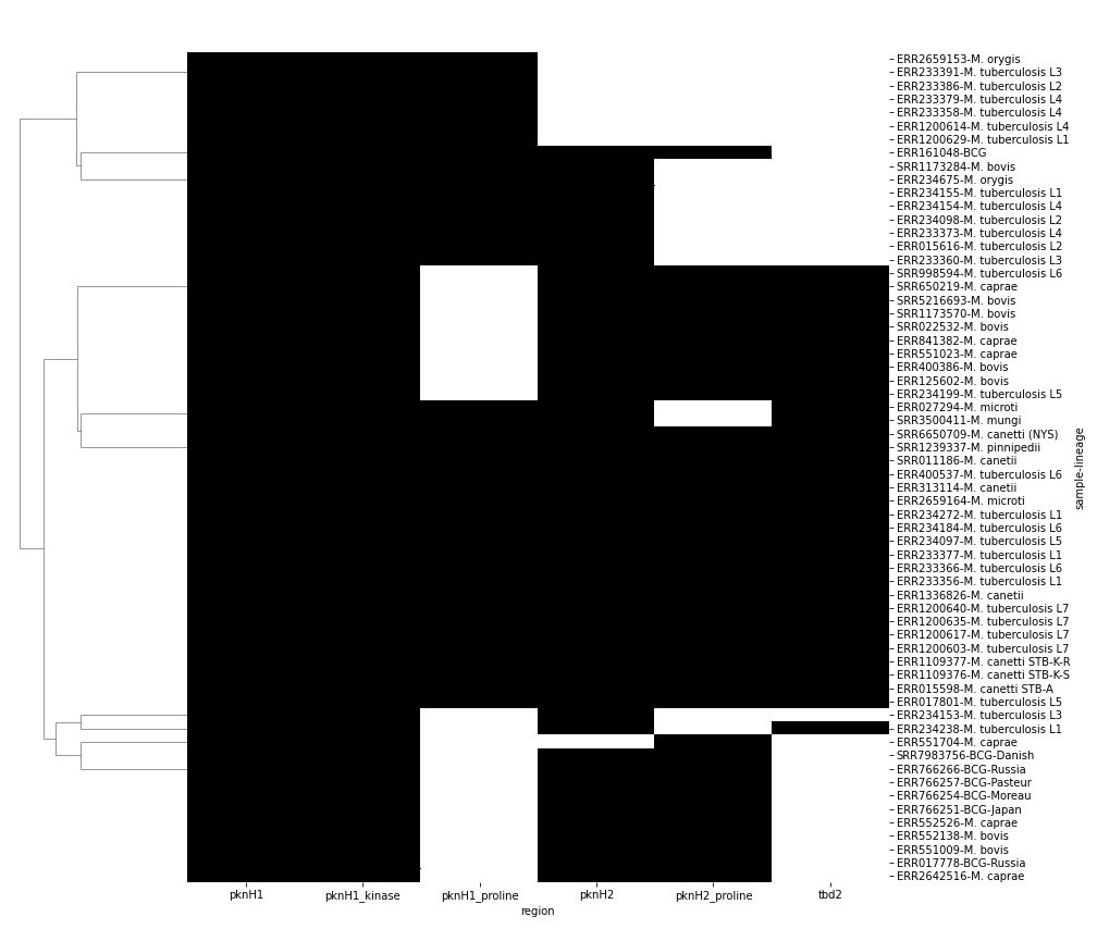
Presence/absence matrix for features inside the locus.