An updated convenience function for ggtree with heatmaps

May 30 2024

Background

Previously we looked at a convenience function for drawing and colouring phylogenetic trees with ggtree. This post contains an updated version of this function with some improvements. Recall that the appropriate meta data is provided as a data.frame object with row names matching tip names of the tree. The first column in cols is used for the tip colors. You also need to provide corresponding cmap values for the colormaps. Numeric data is just coloured with a predefined gradient. This could be further improved. There are lots of other ggtree options and you can’t put everything into one function but this example could be used to expand your own version. See bottom for example usage of the function.

Code

library("ape")
library(RColorBrewer)
library(dplyr)
library('ggplot2')
library('ggtree')
library(tidytree)
library(ggnewscale)

gettreedata <- function(tree, meta){
    d<-meta[row.names(meta) %in% tree$tip.label,]
    d$label <- row.names(d)
    y <- full_join(as_tibble(tree), d, by='label')
    y <- as.treedata(y)
    return(y)
}

get_color_mapping <- function(data, col, cmap){
    labels <- (data[[col]])
    names <- levels(as.factor(labels))
    n <- length(names)
    if (n<10){
        colors <- suppressWarnings(c(brewer.pal(n, cmap)))[1:n]
    }
    else {
        colors <- colorRampPalette(brewer.pal(8, cmap))(n)
    }
    names(colors) = names
    return (colors)
}

ggplottree <- function(tree, meta, cols=NULL, colors=NULL, cmaps=NULL, layout="rectangular",
                       offset=10, tiplabel=FALSE, tipsize=3, tiplabelsize=5, tiplabelcol=NULL,
					   align=FALSE, tipoffset=0) {

    y <- gettreedata(tree, meta)
    if (layout == 'cladogram'){
        p <- ggtree(y, layout='c', branch.length='none')
    }
    else {
        p <- ggtree(y, layout=layout)
    }

    if (is.null(cols)) {
        if (tiplabel){
            p <- p + geom_tiplab(size=tiplabelsize,offset=tipoffset)
        }
        return (p)
    }
    col <- cols[1]
    if (!is.null(colors)) {
        #use predefined colors
        clrs <- colors
    }
    else {
        #calculate colors from cmap
        cmap <- cmaps[1]
        df <- meta[tree$tip.label,][col]
        clrs <- get_color_mapping(df, col, cmap)
    }
    #print (clrs)
    p <- p + new_scale_fill() +
            geom_tippoint(mapping=aes(fill=.data[[col]]),size=tipsize,shape=21,stroke=0) +
            scale_fill_manual(values=clrs, na.value="black")

    p2 <- p
    if (length(cols)>1){
        for (i in 2:length(cols)){
            col <- cols[i]
            if (length(cmaps)>=i){
                cmap <- cmaps[i]
            }
            else {
                cmap = 'Greys'
            }
            df <- meta[tree$tip.label,][col]
            type <- class(df[col,])
            print (type)
            p2 <- p2 + new_scale_fill()
            p2 <- gheatmap(p2, df, offset=i*offset, width=.08,
                      colnames_angle=0, colnames_offset_y = .05)
            if (type %in% c('numeric','integer')){
				p2 <- p2 + scale_fill_gradient(low='#F8F699',high='#06A958', na.value="white")
            }
            else {
                colors <- get_color_mapping(df, col, cmap)
                p2 <- p2 + scale_fill_manual(values=colors, name=col, na.value="white")
            }
        }
    }

    p2 <- p2 + theme_tree2(legend.text = element_text(size=20), legend.key.size = unit(1, 'cm'),
                        legend.position="left", plot.title = element_text(size=40))
            guides(color = guide_legend(override.aes = list(size=10)))
    if (tiplabel) {
		if (!is.null(tiplabelcol)) {
			p2 <- p2 + geom_tiplab(mapping=aes(label=.data[[tiplabelcol]]),
								size=tiplabelsize, align=align,offset=tipoffset)
		}
		else {
        	p2 <- p2 + geom_tiplab(size=tiplabelsize, align=align,offset=tipoffset)
		}
    }
    return(p2)
}

Usage

First we can create some test data using these functions:

# Function to generate a random tree with n tips
generate_tree <- function(n) {
  # Generate the tree using rtree function
  tree <- rtree(n)
  # Generate tip labels from A-Z, then AA, AB, etc. if n > 26
  generate_labels <- function(n) {
    letters <- c(LETTERS, sapply(LETTERS, function(x) paste0(x, LETTERS)))
    return(letters[1:n])
  }
  tip_labels <- generate_labels(n)
  # Assign the generated tip labels to the tree
  tree$tip.label <- tip_labels
  return(tree)
}

generate_metadata <- function(tip_labels) {
  species <- c("Cow", "Sheep", "Deer")
  countries <- c("Ireland", "UK")
  n <- length(tip_labels)
  # Create a data.frame with random metadata
  metadata <- data.frame(
    species = sample(species, n, replace = TRUE),
    year = sample(2000:2020, n, replace = TRUE),
    country = sample(countries, n, replace = TRUE)
  )
  # Add the tip labels as the first column
  rownames(metadata)<-tip_labels
  return(metadata)
}

#create tree and table
tree <- generate_tree(20)
df <- generate_metadata(tree$tip.label)

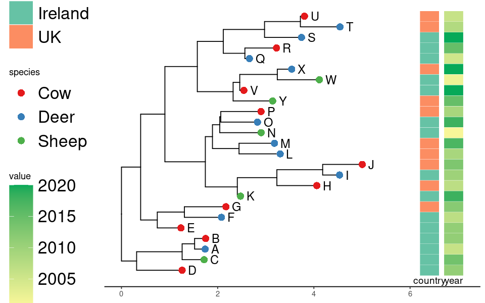
Simple rect layout and three columns of data

Note that offset is according to the tree scale and has to be adjusted manually.

ggplottree(tree, df, layout='rect', cols=c('species','country','year'),
           cmaps=c('Set1','Set2','Blues'), tiplabel=TRUE, tipoffset=.1, tipsize=4, offset=.5)

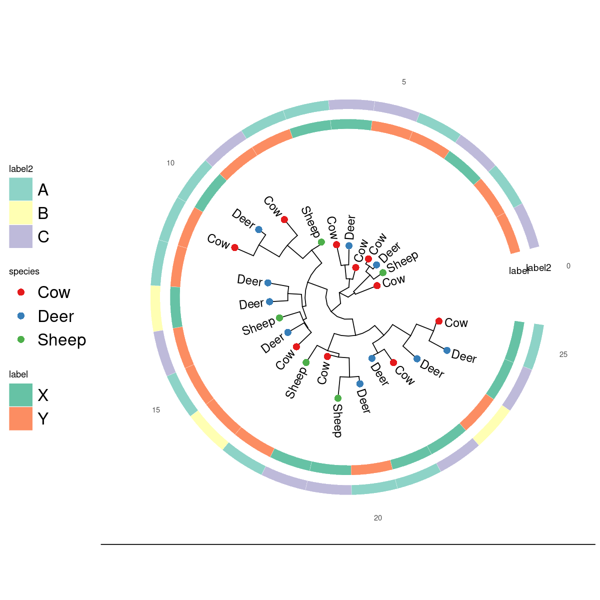
Circular tree with different tip labels

ggplottree(tree, df, layout='c', cols=c('species','label','label2'),
           cmaps=c('Set1','Set2','Set3'), tipsize=4,
           tiplabel=TRUE, tiplabelcol='species', tipoffset=.2, offset=.8 )

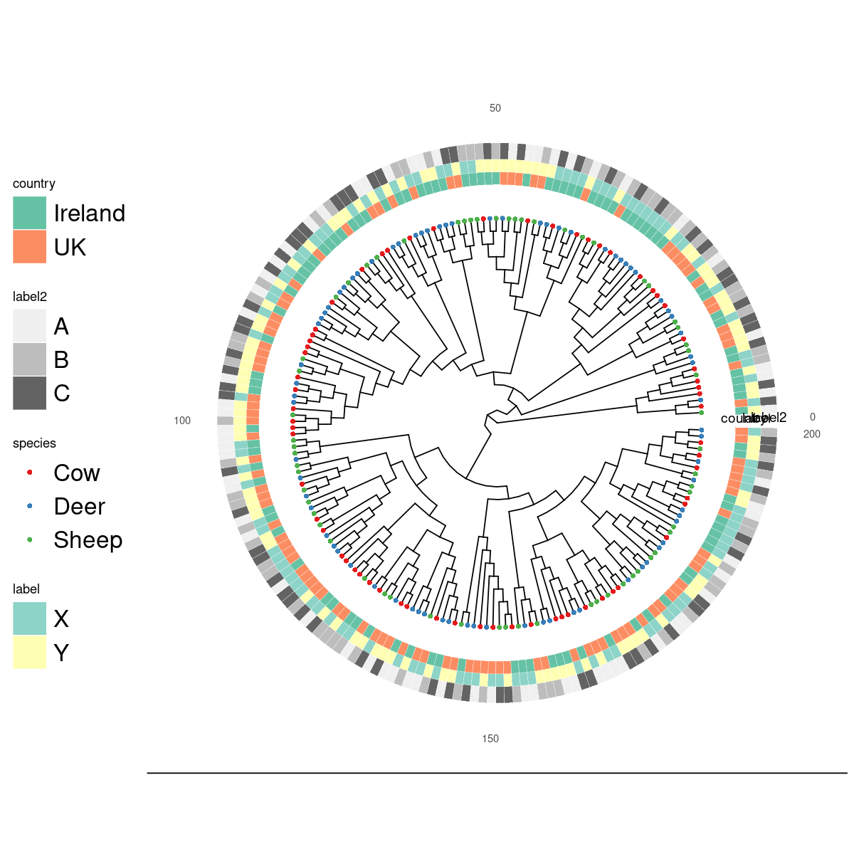
Cladogram with multiple color scales

This example has more tips. A cladogram just removes the branch lengths. It’s not actually a ggtree layout name. If you provide no color scale a grayscale one is used.

ggplottree(tree, df, layout='cladogram', cols=c('species','country','label','label2'),
           cmaps=c('Set1','Set2','Set3',NULL), tipsize=3, offset=1 )