Using IGV inside Jupyter Lab notebooks
Background
IGV is a popular Java based genome browser. You can install IGV in linux with a package manager such as using apt in Ubuntu or download the binary. Jupyter notebooks are browser based environments for Python programming with a lot of additional libraries that add functionality. Widgets can also be used. IGV also uses the igv.js javascript file to implement browser embedding. This also allows it to be used in Jupyter Lab by using the igv-jupyterlab package. Install using:
pip install igv-jupyterlab
You should restart the jupyter server after doing this.
Code
Below is shown how to display a local reference genome against local aligned bam files. The reference here is Mycobacterium Tuberculosis. Most important is to get the urls correct for loading local files. You need to use the url of the notebook server as a prefix along with /files and then specify the local path. The files need to be in the same folder as where you are running Jupyter Lab. You can add gff, vcf, bam and bed files as tracks and specify a height, color and other properties. Here the method is to populate a track list and then provide that as an argument when creating the genome object with the create_genone helper function. As with any browser you have to zoom in below a certain level to see details, especially the alignment tracks.
from igv_jupyterlab import IGV

url = 'http://localhost:8890/files/'

bams={'m.caprae':'results_mtb/mapped/ERR552526.bam',
      'm.microti':'results_mtb/mapped/ERR027294.bam',
      'm.bovis':'results_mtb/mapped/59-6110.bam'}

#populate a list of tracks, first we add the gff
track_list = [{"name": "MTB-H37Rv",
                "url": url+"results_mtb/MTB-H37Rv.gb.gff",
                "format": "gff",
                "type": "annotation",
                "height":120,
                "indexed": False }
             ]

colors=['orange','green','gray']
i=0
#add a bam for each of the files above
for b in bams:
    d = {"name": b,
        "url":url+bams[b],
        "type": "alignment",
         "displayMode":"SQUISHED",
         "height":130,
         "removable":True,
         "color":colors[i],
        "indexed": True }
    track_list.append(d)
    i+=1

#create the genome object with reference and tracks
genome = IGV.create_genome(
    name="MTB-H37Rv",
    fasta_url=url+'MTB-H37Rv.fa',
    index_url=url+'MTB-H37Rv.fa.fai',
    tracks=track_list
)

#create the widget
igv = IGV(genome=genome)
#zoom to a region
igv.search_locus('NC_000962.3', 1695281,  1708539)
#show in cell
display(igv)
Result
The resulting view is below. When zoomed out enough, the viewer is slower than the desktop version to render alignment tracks which may be annoying. It may be more useful for showing pre-calculated co-ordinates and saving as images. You can view an svg image of the viewer using igv.get_svg() however I couldn’t get this to work.
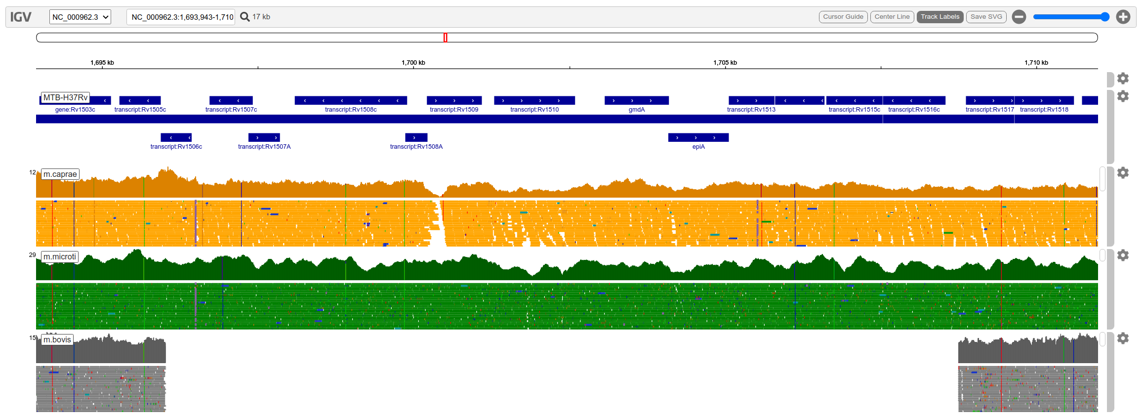
Region showing deletion in M.bovis genome.