wgMLST vs the reference-align-SNP-calling method for M.bovis
Background
We previously showed an implementation of whole genome MLST (Whole genome Multi Locus Sequene Typing) for bacterial genotyping. This was implemented with the example of M.bovis. Here we show a comparison with the traditional method of reference alignment then SNP calling for recreating a phylogeny for a group of related isolates. The MLST method here is used on the consensus sequences derived from the multi sample vcf file of a previous variant calling run with SNiPgenie (another pipeline could be used too). The Jupyter notebook with this code is here. First we generate artificial reads from a simulated phylogeny, then compare the resulting trees calculated from both methods.
Simulating sequence data
To create a reasonable test set, we can simulate a set of related sequences of M.bovis. To do this we first create a simulated outbreak using transphylo, an R package. This generates a phylogeny which is used as input to a sequence simulator that takes the newick file and produces simulated genome sequences along the tree by adding SNPs. Here I have used phastSim, since it was easiest for me to get working.
For making the outbreak, I used settings from Walter et al.. This is the R code:
library(ape)
library(phangorn)
library('TransPhylo')

set.seed(1)
neg=100/365
off.r=3
w.shape=10
w.scale=0.1
pi=0.4
simu <- simulateOutbreak(neg=neg,pi=pi,off.r=off.r,w.shape=w.shape,
                         w.scale=w.scale,dateStartOutbreak=2005,dateT=2009)
plot(simu)
ttree<-extractTTree(simu)
ptree<-extractPTree(simu)
plot(ptree)
p<-phyloFromPTree(ptree)
plot(p)
axisPhylo(backward = F)
write.tree(p,'sim.newick')
Simulated outbreak from TransPhylo.
Transmission tree.
We then use the newick file to make sequences with phastSim as follows. The scale argument can be seen as the fraction of the genome length to mutate. It can be set so as to generate a specific range of SNPs across the phylogeny. Note that the time scale of the simulation is not that important here as we are mainly concerned with adjusting the number of SNPs to test the methods.
phastSim --outpath simulation_output/ --seed 1 --createFasta --createPhylip --treeFile sim.newick --scale 6.9e-07 --invariable .1 --alpha 1.0 --omegaAlpha 1.0 --reference Mbovis_AF212297.fa
This makes a single fasta file with a sequence for each genome. Finally we can make artificial fastq files from these genomes to run in our SNP pipeline. I used ArtificialFastqGenerator for this. To make this faster I wrapped the call in a Python method and ran it in parallel for all sequences using joblib. (This program uses a lot of memory so be careful when using more than one core). generate_fastqs will parse the input fasta file and make fastqs for each sequence, these are made as paired end reads of 150 bp each. The other settings shown in the make_fastq method are explained in the ArtificialFastqGenerator documentation.
import subprocess

def make_fastq(ref, outfile, cmp=100):

    f1 = '/storage/btbgenie/mbovis_ireland/Wicklow/Fastqs_07-01-18/17-MBovis_S21_L001-4_R1_001.fastq.gz'
    f2 = '/storage/btbgenie/mbovis_ireland/Wicklow/Fastqs_07-01-18/17-MBovis_S21_L001-4_R2_001.fastq.gz'
    cmd = 'java -jar /local/ArtificialFastqGenerator/ArtificialFastqGenerator.jar -O {o}'\
          ' -R {r} -S ">temp" -RL 150 -CMP {cmp} -CSD 0.2 -SE true'.format(r=ref, o=outfile,cmp=cmp,f1=f1,f2=f2)
    subprocess.check_output(cmd, shell=True)
    return

def generate_fastqs(infile, outpath):

    from joblib import Parallel, delayed
    import time
    num_cores = 4

    simrecs = list(SeqIO.parse(infile,'fasta'))
    def my_func(rec):
        from tempfile import mkstemp
        x,tmp = mkstemp()
        SeqIO.write(SeqRecord(rec.seq,id='temp'), tmp, 'fasta')
        out = os.path.join(outpath,rec.id)
        make_fastq(tmp, out)

    st = time.time()
    Parallel(n_jobs=num_cores)(delayed(my_func)(i) for i in simrecs)
    print (time.time()-st)
    cmd = 'pigz %s/*.fastq' %outpath
    subprocess.check_output(cmd, shell=True)

#run
generate_fastqs('sim_seqs.fa', 'sim_fastq')
Running the test
We can now test the two methods by first running SNiPgenie on the simulated reads. This makes a vcf file which is used by the wgMLST tool to make consensus sequences and then run it’s analysis on them. This will not give quite the same as using a de novo assembly but it is faster and for our purposes here is sufficient. SNiPgenie will build a maximum likelihood tree from the core (variant sites) alignment using RaXML, which is saved to the results folder. Once read back in we can plot it with toytree. The MLST tree is derived from the distance matrix of the allele values. We can see the branch lengths may differ but the placement of nodes is the same between the two approaches. Both trees are consistent with the transmission tree shown above. However, this example had about 500 snps between all the samples which is quite a large diversity for this species and would reflect a longer time scale.
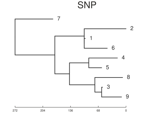
ML tree from the SNP method with scale shown as number of SNPs.
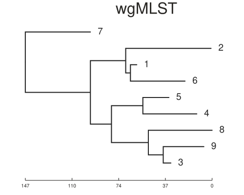
NJ tree from the wgMLST method, scale is allele distance.
#run snipgenie
import snipgenie
from pathogenie import app
import toytree

args = {'threads':10, 'outdir': 'sim_results', 'labelsep':'_',
        'input':['sim_fastq/'], 'overwrite':True,
         'species':'Mbovis-AF212297',
         'custom_filters': True,
         'buildtree':True}
W = snipgenie.app.WorkFlow(**args)
st = W.setup()
W.run()

tresnps = toytree.tree('sim_results/tree.newick')
tresnps=tresnps.root('1')
tresnps=tresnps.drop_tips('ref')
canvas,t,r=tresnps.draw(layout='r',scalebar=True,height=400,width=500)
sd=snpdist = pd.read_csv('sim_results/snpdist.csv',index_col=0).iloc[1:,1:]
print (sd)

#run MLST using the vcf from above to make consensus sequences
sim_vcf = 'sim_results/filtered.vcf.gz'
simprofs = run_samples(sim_vcf, 'sim_mlst', threads=12)

D = dist_matrix(simprofs)
print (D)
D.to_csv('dist_mlst.csv')
treefile='mlst.newick'
tree_from_distmatrix(D, treefile)
tremlst = toytree.tree(treefile)
tremlst=tremlst.root('1')
canvas,t,r=tremlst.draw(layout='r',scalebar=True,height=400,width=500)
Closely related isolates
On the time scale of the simulation above ~500 SNPs between isolates is not realistic. Another set was simulated with about 20 SNPs variation in total. This is a better test of the methods. The trees below show the results for this case and now the trees are different. You will notice that the basic structure of the phylogeny is retained for the SNP tree but errors are now present in the placement of samples on the MLST tree. For example samples 1 and 5 are now in the same sub-clade as 8, 3 and 9. We can also estimate the normalised tree distances to the refrence phylogeny using the TreeDist package in R. These are 0.37 and 0.65 for the SNP and wgMLST respectively. This indicates a lower sensitivity for the wgMLST method with small differences between isolates. It should be underlined that the trees are arrived somewhat differently, with the ML tree from SNP alignment being created using a substitution model.
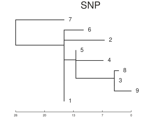
ML tree from the SNP method with scale shown as number of SNPs.
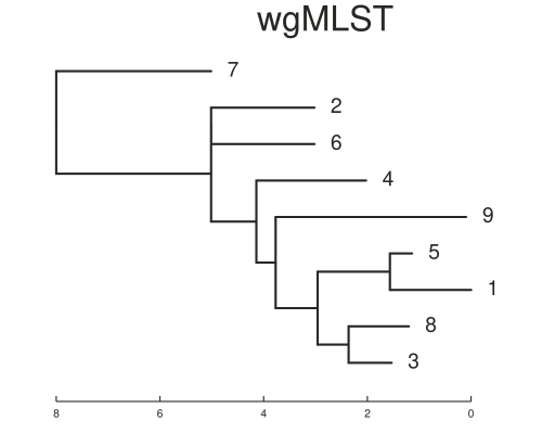
NJ tree from the wgMLST method, scale is allele distance.
We can also see that sometimes the MLST method indicates larger distances between isolates. This is because any difference between each sequence is counted, whereas only non-synonymous SNPs are being counted in the SNP calling method. That is indicated in the distance matrices below from both methods. This is a rough comparison and not meant to be definitive. As discussed previously whole genome MLST has it’s own advantages and applications.
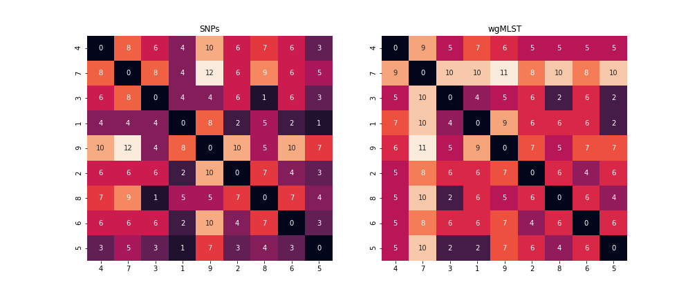
Pairwise distance matrix for both methods.
Links
- MLST revisited: the gene-by-gene approach to bacterial genomics
- Harmonized Genome Wide Typing of Tubercle Bacilli Using a Web-Based Gene-By-Gene Nomenclature System
- The ‘inaccuracy’ of phylogenies based on whole genome SNPs identified by mapping to a reference
- toytree
References
- phastSim: efficient simulation of sequence evolution for pandemic-scale datasets. Nicola De Maio, Lukas Weilguny, Conor R. Walker, Yatish Turakhia, Russell Corbett-Detig, Nick Goldman. bioRxiv 2021.03.15.435416; doi: https://doi.org/10.1101/2021.03.15.435416
- Genomic variant-identification methods may alter Mycobacterium tuberculosis transmission inferences. Katharine S. Walter et al. Microbial Genomics, 31 July 2020; https://doi.org/10.1099/mgen.0.000418