Make networkx Delaunay graphs from geopandas dataframes
Background
Geopandas Geodataframes store spatial data such as points and polygons. This post adapts code a from some examples online to show how to convert spatial points into a Delaunay graph. This is a undirected graph with edges between adjacent points only. This may be useful for building a spatial contact network of neighbouring points and doing further processing. Here we convert into networkx graphs.
First we make a GeoDataFrame from some random points:
def random_points(n):
    import random
    # Create an empty GeoDataFrame
    gdf = gpd.GeoDataFrame(columns=['geometry'])

    # Generate n random points and add them to the GeoDataFrame
    for i in range(n):
        x = random.uniform(-180, 180)
        y = random.uniform(-90, 90)
        point = Point(x, y)
        temp_gdf = gpd.GeoDataFrame(geometry=[point])
        temp_gdf['name']='A'
        gdf = pd.concat([gdf,temp_gdf])

    gdf.crs = {'init': 'epsg:4326'}
    return gdf
The voronoi cells are shown also. These are used to compute the graph.
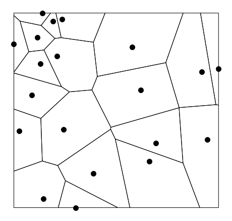
Random points.
Method 1
We now want to compute the Delaunay graph for these points, first using scipy. This is shown below. There is also code to add a name field to each node in case we want to use such identifiers to match back to the dataframe in a more useful manner.
import sys,os
import numpy as np
import pandas as pd
import geopandas as gpd
import networkx as nx
from shapely.geometry import Point, LineString, Polygon, MultiPolygon

def delaunay_scipy(gdf, key='name'):
    """Get delaunay graph from gdf of points using scipy"""

    from scipy.spatial import Delaunay
    from itertools import combinations

    pos = {i: (gdf.iloc[i].geometry.x, gdf.iloc[i].geometry.y) for i in range(len(gdf))}
    gdf['x'] = gdf.geometry.x
    gdf['y'] = gdf.geometry.y
    # Create a Delaunay triangulation of the points
    tri = Delaunay(gdf[['x', 'y']])

    # Create a Graph from the Delaunay triangulation
    G = nx.Graph()
    G.add_nodes_from(range(len(gdf)))

    for simplex in tri.simplices:
        G.add_edges_from(combinations(simplex, 2))
    for i, node in enumerate(G.nodes()):
        G.nodes[node]['name'] = gdf.iloc[i][key]
    nx.set_node_attributes(G, pos, 'pos')
    return G,pos
Method 2
An alternative method is to use pysal modules. This gets the x-y coordinates into a numpy array. The voronoi polygons (cells) are calculated and we construct the adjacency graph between them using ‘Rook’ contiguity. This code is explained in more detail here. Note that the cells/polygons are clipped using the bounding box of the points before the graph is made (shown above). We can also use clip=convex_hull.
def delaunay_pysal(gdf, key='name'):
    """Get delaunay graph from gdf of points using libpysal"""

    from libpysal import weights, examples
    from libpysal.cg import voronoi_frames

    coordinates = np.column_stack((gdf.geometry.x, gdf.geometry.y))
    cells, generators = voronoi_frames(coordinates, clip="extent")
    delaunay = weights.Rook.from_dataframe(cells)
    G = delaunay.to_networkx()
    positions = dict(zip(G.nodes, coordinates))
    nx.set_node_attributes(G, positions, 'pos')
    #add names to nodes
    for i, node in enumerate(G.nodes()):
        G.nodes[node]['name'] = gdf.iloc[i][key]
    return G, positions
The reason we return the positions in both cases is so we can plot the graphs consistent with the spatial plot above and to compare them.
fig,ax=plt.subplots(1,2,figsize=(14,10))
axs=ax.flat
G,pos=delaunay_scipy(rand, key='label')
nx.draw(G, pos, node_size=500, node_color='y', with_labels=True,ax=axs[0])
G,pos=delaunay_pysal(rand, key='label')
nx.draw(G, pos, node_size=500, node_color='y', with_labels=True,ax=axs[1])
Results from both are shown below. They are almost identical except you can see the second method is missing some of the outer edges. This may be related to the clipping that voronoi_frames does in order to make the cells. However this looks more correct as the fist method is connecting outer nodes very far apart.
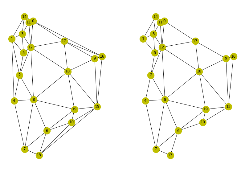
Results of methods 1 and 2.
How is this useful
This type of graph is used in things like community detection. We can use the resultant graph to examine nodes for those adjacent to it for example. In the snippet below we get the name of node 0 and those of all the nodes connected to it.
name=G.nodes[0]['name']
conn = G[0]
names = [G.nodes[c]['name'] for c in conn ]