Plot phylogenies with annotation in R using ggtree and gheatmap
Background
There are many online examples of how to draw phylogenetic trees using various R tools. One is ggtree, based on the ggplot packages, which provides a wide range of options. This example shows how to write some functions that can plot trees with an arbitrary number of heatmap annotations, given the appropriate meta data in a data.frame object. The columns to be used are provided as a list along with color maps for each. The first column is used for the tip colors. Note that you will see a warning: “Scale for ‘fill’ is already present. Adding another scale for ‘fill’, which will replace the existing scale.” when this is run but it can be ignored. This is because a new scale_fill_manual is called each time we add a heatmap. There is also some code here to deal with the case of continuous column types, in which case scale_color_brewer is used instead.
See here for an updated version of the function.
Code
library("ape")
library(RColorBrewer)
library(dplyr)
library('ggplot2')
library('ggtree')
library(tidytree)
library(ggnewscale)

gettreedata <- function(tree, meta){
    #get treedata object
    d<-meta[row.names(meta) %in% tree$tip.label,]
    d$label <- row.names(d)
    y <- full_join(as_tibble(tree), d, by='label')
    y <- as.treedata(y)
    return(y)
}

get_color_mapping <- function(data, col, cmap){
    labels <- (data[[col]])
    names <- levels(as.factor(labels))
    n <- length(names)
    if (n<10){
        colors <- suppressWarnings(c(brewer.pal(n, cmap)))[1:n]
    }
    else {
        colors <- colorRampPalette(brewer.pal(8, cmap))(n)
    }
    names(colors) = names
    return (colors)
}

ggplottree <- function(tree, meta, cols=NULL, cmaps=NULL, layout="rectangular",
                       offset=10, tiplabel=FALSE, tipsize=3) {

    y <- gettreedata(tree, meta)
    p <- ggtree(y, layout=layout)
    if (is.null(cols)){
        return (p)
    }

    col <- cols[1]
    cmap <- cmaps[1]
    df<-meta[tree$tip.label,][col]
    colors <- get_color_mapping(df, col, cmap)

    #tip formatting
    p1 <- p + new_scale_fill() +
          geom_tippoint(mapping=aes(fill=.data[[col]]),size=tipsize,shape=21,stroke=0) +
          scale_fill_manual(values=colors, na.value="white")

    p2 <- p1
    if (length(cols)>1){
        for (i in 2:length(cols)){
            col <- cols[i]
            cmap <- cmaps[i]
            df <- meta[tree$tip.label,][col]
            type <- class(df[col,])
            p2 <- p2 + new_scale_fill()
            p2 <- gheatmap(p2, df, offset=i*offset, width=.08,
                      colnames_angle=0, colnames_offset_y = .05)
            #deal with continuous values
            if (type == 'numeric'){
                p2 <- p2 + scale_color_brewer(type="div", palette=cmap)
            }
            else {
                colors <- get_color_mapping(df, col, cmap)
                p2 <- p2 + scale_fill_manual(values=colors, name=col)
            }
        }
    }

    p2 <- p2 + theme_tree2(legend.text = element_text(size=20), legend.key.size = unit(1, 'cm'),
                        legend.position="left", plot.title = element_text(size=40))
            guides(color = guide_legend(override.aes = list(size=10)))

    return(p2)
}
Usage
A simple tree and meta data are created in the code below for illustration. We then plot by calling the above function.
tree <- ape::read.tree(text='((A, B), ((C, D), ((E, F), (G, H))));')
options(repr.plot.width=8, repr.plot.height=6)
df <- data.frame (name = c('A','B','C','D','E','F','G','H'),
                  label1 = c('X','X','Y','Y','Y','Y','Y','X'),
                  species = c('dog','cat','dog','dog','cat','cat','cat','cat'),
                  country = c('Ireland','Ireland','France','UK','France','UK','France','UK'),
                  year = c(2013,2014,2015,2015,2017,2012,2012,2013)
                  )
row.names(df) <- df$name
ggplottree(tree, df, cols=c('label1','species','country'),
           cmaps=c('Set1','Set2','Set3'), tipsize=8, offset=.5 ,layout='rect')
Which makes a table like this to use as the label data:
name	label1	species	country year
A	X	dog	Ireland	2013
B	X	cat	Ireland	2014
C	Y	dog	France	2015
D	Y	dog	UK	2015
E	Y	cat	France	2017
F	Y	cat	UK	2012
G	Y	cat	France	2012
H	X	cat	UK	2013
Finally, the tree looks like this:
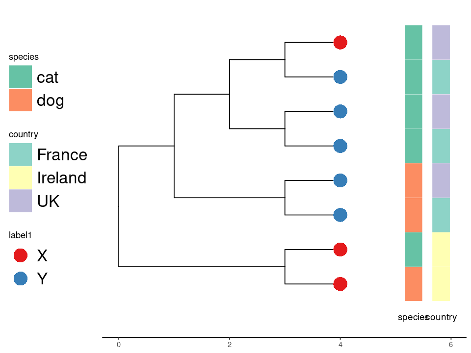
Example tree.
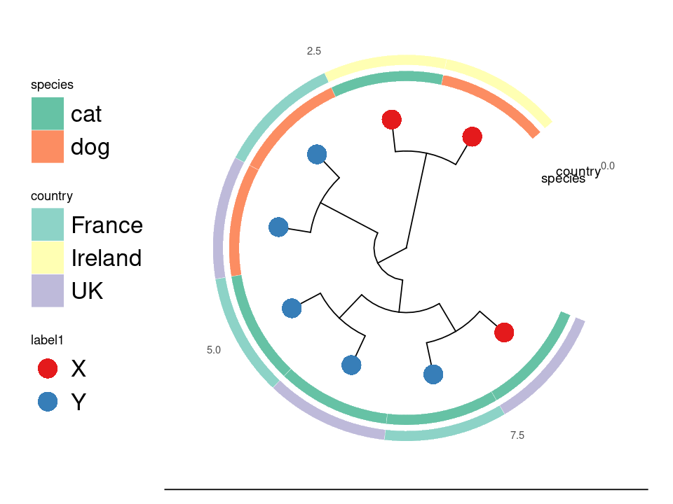
Circular layout.
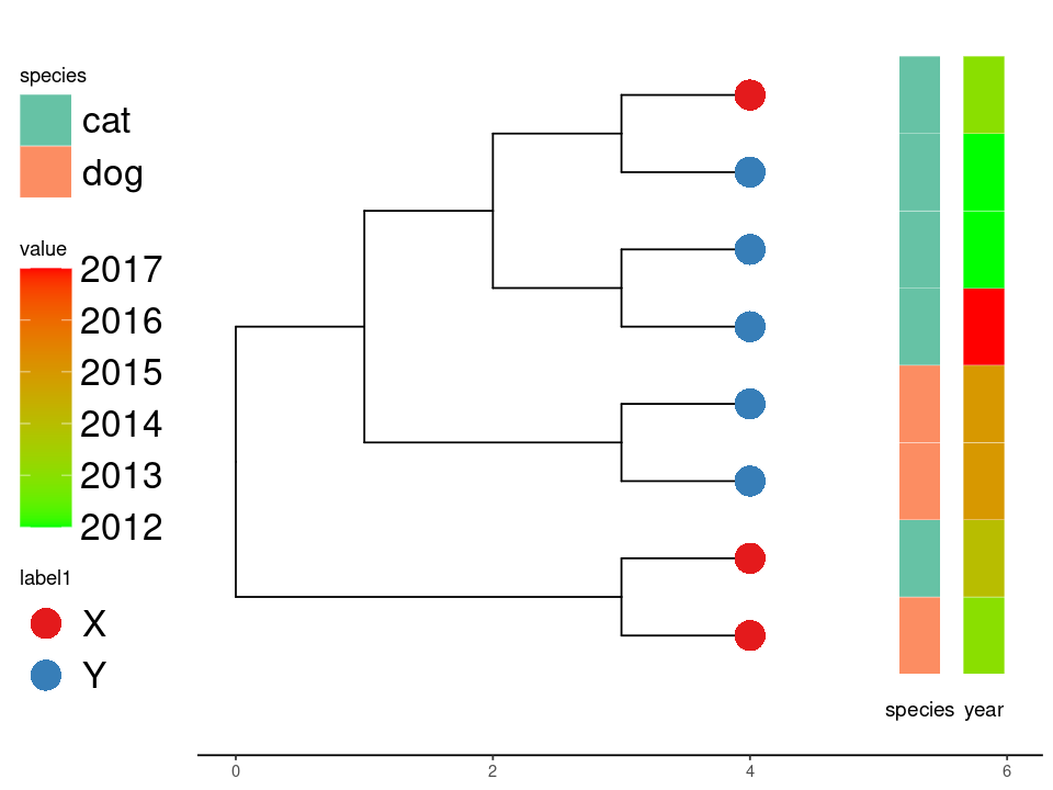
Continuous values.
Links
- https://yulab-smu.top/treedata-book/chapter10.html