Plotting gridded quantitative data with geopandas - Irish forestry
Background
A previous post showed how to create grids over polygons using geopandas. To make practical use of this requires you have some kind of quantitative data that you want to bin into each grid polygon. This could be a summary statistic over that area derived from a more fine grained spatial dataset. To do this we would combine the grid with the original data using sjoin and then aggregate using dissolve with some defined aggregating function. sjoin is like merging in pandas except it’s joining GeoDataFrames based on spatial overlaps.
In this example we will use data on tree coverage in Ireland. We want to summarise the coverage values over the grid instead of just by county. Below, we load the shapefiles and spatial join the original data to the grid, the use dissolve to get the aggregated area values for all polygons in each grid cell.
import geopandas as gpd
forests = gpd.read_file('forestry_data/landuse_forests.shp')
forests = forests.to_crs("EPSG:3857")
woods = gpd.read_file('forestry_data/natural_wood.shp')
woods = woods.to_crs("EPSG:3857")
total = pd.concat([forests,woods])
total['area'] = total.to_crs('EPSG:6933').geometry.area/10**6

def grid_summary(gdf, data, n_cells=20):
    """Get grid summary from a map and associated meta data"""

    cols=['geometry','NAME_TAG']
    #get grid
    grid = create_hex_grid(gdf, n_cells=n_cells, overlap=True, crs="EPSG:3857")[cols]
    #get centroids as alternative to polygons
    cent = data.copy()
    cent.geometry = data.centroid
    #sjoin merges on spatial overlap
    merged = gpd.sjoin(cent, grid, how='inner', predicate='intersects')
    #aggregate
    dissolve = merged.dissolve(by="index_right", aggfunc='sum')
    #assign column to area sums
    grid.loc[dissolve.index, 'value'] = dissolve['area'].values
    return grid
Results
To test the method works it’s easier to take a smaller area like a county to test on. Below we run the method on county Wicklow data and overlay the original polygons of tree areas onto the grid coloured by the summary values of total square area. Note that there are various ways to bin the polygons into each cell for the area calculation. The most naive is to just find all polygons overlapping the cell. Or we can take the centroids of each and use them for the sjoin. The latter avoids duplication of polygons being assigned to multiple adjoining cells. I do not know which is most optimal but the centroid method seems more sensible. Either method will be less accurate the smaller the cells. Both are shown below with the original polygons overlaid. The most accurate method would be to just use a custom aggregation function that clips everything within each cell and calculates that area. I didn’t get time to do that here.
wicklow = total[total.county.isin(['Wicklow'])]
wc = counties[counties.NAME_TAG=='Wicklow']
gdf = grid_summary(wc, wicklow, n_cells=10)
fig,ax=plt.subplots(1,1,figsize=(12,12))
gdf.plot(column='value',ec='black',lw=0.2,legend=True, cmap='Reds',alpha=0.9,
          legend_kwds={'label': "Tree coverage (square km)", "shrink": .6},
          ax=ax)
wicklow.plot(fc='black',lw=.5,ax=ax,alpha=0.6)

ax.axis('off')
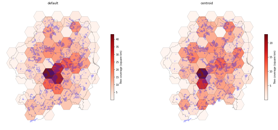
Example for one county.
Ireland
Finally we can apply this method to the whole dataset for the country:
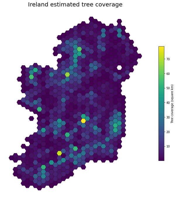
Tree coverage over country.